A Comprehensive Guide on Geostationary Orbit Equation

Introduction to Geostationary orbit equation

The concept of a geostationary orbit is a cornerstone of modern satellite technology. This unique orbital path allows satellites to hover over a single point on Earth, enabling continuous communication, weather observation, and television broadcasting. To understand how this is possible, we must explore the geostationary orbit equation, calculate the radius of geostationary orbit, and see how these concepts are applied in real-world systems.

What Is a Geostationary Orbit?

A geostationary orbit is a type of circular orbit located directly above Earth’s equator. In this orbit, a satellite rotates at the same speed as the Earth, which makes it appear stationary to observers on the ground. As reported also in ESA article, the satellite moves with a speed that exactly match Earth’s orbit rotation, taking 23 hours 56 minutes and 4 seconds to complete one period.

*Illustration of Earth with a satellite in geostationary orbit directly above the equator, matching Earth’s rotation.*

Due to the high altitude, satellites in GEO can cover a large portion of Earth. Three evenly spaced satellites can provide near-global coverage, instead the lower the altitude the greater the number of satellites.

What is important to highlight is that geostationary orbits are particular geosynchronous orbit. A geosynchronous orbit (GEO) is a prograde, low inclination orbit about Earth having a period of 23 hours 56 minutes 4 seconds (sidereal day). The spacecraft returns to the same point in the sky at the same time each day.

Instead, to achieve a geostationary orbit, a geosynchronous orbit is chosen with an eccentricity of zero, and an inclination of either zero, right on the equator. Geostationary orbit (also called GEO) is ideal for satellites that need to stay fixed above a specific location, such as telecommunication satellites, allowing antennas on Earth to stay in a constant position, always pointing at the satellite. It is also valuable for weather satellites, enabling continuous monitoring specific regions to track evolving weather patterns over times and see how weather trends emerge.

Below, we are providing a brief table to show the differences between geosynchronous and geostationary orbits.

Feature	Geosynchronous	Geostationary
Orbital period	≈ 23h 56m (sidereal day)	≈ 23h 56m (sidereal day)
Orbit shape	Can be elliptical or circular	Must be circular
Inclination	Any inclination (0° to ~63°)	0° (equatorial)
Ground track	Forms a figure-8 or loop in the sky	Appears fixed above the equator
Motion	Satellite appears to move relative to Earth	Satellite appears stationary to an observer
Use cases	Reconnaissance, scientific, some comsats	TV, weather satellites, communications (e.g. TV)

The Geostationary Orbit Equation

As discussed before, a geostationary orbit has the following characteristics:

23h 56m 4s period;
Circular orbit, zero eccentricity (e=0);
zero inclination with respect to equatorial plane (i=0).

Starting from the generic orbit equation:

$\begin{equation*} r = \frac{h^2}{\mu} \frac{1}{1+e \cdot \cos(\theta)} \end{equation*}$

With the proper substitution, it is possible to retrieve that:

$\begin{equation*} r = \frac{h^2}{\mu} \end{equation*}$

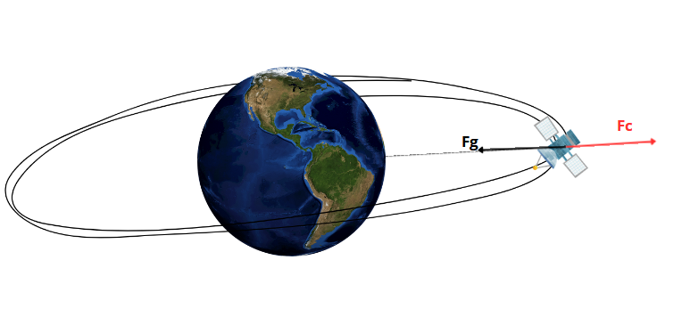
Therefore, it is clear that we are talking about a circular orbit (as shown in picture below, where Gravity is pulling the satellite inward and centripetal force keep it in orbit.). Starting from force balance:

$\begin{equation*} F_g = F_c \end{equation*}$

$\begin{equation*} G \frac{m \cdot M}{r^2} = \omega^2 r m\end{equation*}$

$\begin{equation*} v_{\perp} = \sqrt{ \frac{GM}{r} } = \sqrt{\frac{\mu}{r}}\end{equation*}$

Where:

G is the gravitational constant (6.674 × 10⁻¹¹ N·m²/kg²)
M is the mass of the Earth (~5.972 × 10²⁴ kg)
m is the satellite mass
r is the radius of geostationary orbit (from Earth’s center)
ω is the angular velocity of the satellite (same as Earth’s rotation)

Calculating the Radius of Geostationary Orbit

To find the correct orbit, we solve for r by combining the equation with the formula for angular velocity:

$\begin{equation*} \omega = \frac{2\pi}{T} \end{equation*}$

Where T is the orbital period. As stated before, the period shall be equivalent to one sidereal day 23h 56m 4s, which means:

$\begin{equation*} 23 \cdot 3600 + 56 \cdot 60 + 4 = 86,164 \ \text{seconds} \end{equation*}$

This is very important, because adding this constraint we are liking the period of rotation of the satellite to the Earth’s orbit rotation. In other words, we are saying that the satellite period shall be equal to 24h Earth’s rotation.

Rearranging the geostationary orbit equation to isolate the radius:

$\begin{equation*} \frac{\mu}{r^2} = \omega^2 r \end{equation*}$

$\begin{equation*} r = \frac{\mu T^2}{4\pi^2} \end{equation*}$

Considering the following values values:

$G = 6.674 \times 10^{-11}$
$M = 5.972 \times 10^{24}$
$T = 86164$ seconds

It is possible to retrieve the radius of geostationary orbit:

$\begin{equation*} r^3 \approx \frac{(6.674 \times 10^{-11})(5.972 \times 10^{24})(86164)^2}{4\pi^2} \approx 42,164 \text{ km} \end{equation*}$

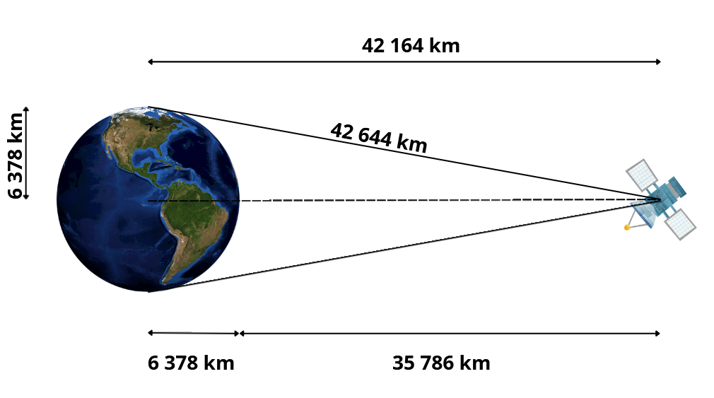
This result gives the geostationary orbit radius from Earth’s center. To find the altitude above Earth’s surface, subtract Earth’s radius (about 6,378 km):

$42,164 \text{ km} - 6,378 \text{ km} = 35,786 \text{ km}$

*The picture shows the radius of geostationary orbit.*

Launching a Geostationary satellite

How is it possible to reach the radius of geostationary orbit? Using Geostationary Transfer Orbit!

When launching satellites into geostationary orbit (GEO), rockets do not send them directly to their final altitude 35,786 km above Earth. Instead, they first place the satellite into an elliptical path known as a Geostationary Transfer Orbit (GTO) — a critical stepping stone in orbital mechanics (see also dedicated chapter here).

A Geostationary Transfer Orbit (GTO) is an elliptical orbit that serves as an intermediate trajectory between low Earth orbit (LEO) or parking orbit and geostationary orbit (GEO). It typically has:

Perigee: ~200–300 km (close to Earth)
Apogee: ~35,786 km (matching the GEO altitude)
Inclination: Often non-zero, depending on launch site latitude

This orbit allows the satellite to coast to its highest point (apogee), where an onboard satellite engine performs a final circularization burn to enter GEO.

Calculating GTO

Circular starting Orbit

To calculate the GTO orbit, we started from a circular orbit at an altitude of 150km. Knowing this, it is possible to retrieve information on angular momentum, orthogonal speed, energy and orbit period. Let’s start from the standard orbit equation:

$\begin{equation*} r = \frac{h^2}{\mu} \frac{1}{1+ e \cos(\theta)} \end{equation*}$

Since, the orbit is circular we can assume $e=0$ . In addition, we can consider also the true anomaly equal to zero ( $\theta = 0$ . Therefore:

$\begin{equation*} r = \frac{h^2}{\mu} \Rightarrow h = \sqrt{r \mu} = 51,010.95 \ \text{km}/\text{s} \end{equation*}$

Therefore, the orthogonal speed can be computed:

$\begin{equation*} v_{\perp} = \frac{h}{r} = 7.814 \ \text{km}/\text{s} \end{equation*}$

The period is computed:

$\begin{equation*} T = \frac{2 \pi r}{v_{\perp}} = \frac{2 \pi r}{\sqrt{\mu/r}} = \frac{2 \pi}{\sqrt{\mu}} \cdot r^{3/2} = 5249.22 \ \text{s} \end{equation*}$

Therefore, the half period is: $T_{1/2} = 2624,61 \ \text{s}$ . In addition, it is possible to compute the energy:

$\begin{equation*} \epsilon = - \frac{1}{2} \frac{\mu^2}{h^2} = -30.529 \ \text{km}^2/\text{s}^2 \end{equation*}$

GTO maneuver

The GTO maneuver requires to enter in an elliptic orbit, with $r_P = 6,528.14 \ \text{km}$ and $r_A = 42,164 \ \text{km}$ with the following semi-major axis:

$\begin{equation*} a = \frac{r_P + r_A }{2} = 24,346.07 \ \text{km}\end{equation*}$

From this it is possible to compute the energy of the orbit:

$\begin{equation*} \epsilon = - \frac{\mu}{2a} = -8.186 \ \text{km}^2/\text{s}^2 \end{equation*}$

Now, considering the energy formula it is possible to compute the speed in the perigee:

$\begin{equation*} \epsilon = \frac{v^2}{2} - \frac{\mu}{r} \Rightarrow v_P = \sqrt{2 \cdot \Big( \epsilon + \frac{\mu}{r_P} \Big)} = 10.2832 \ \text{km}/\text{s} \end{equation*}$

From this it is possible to compute the first burn:

$\begin{equation*} \Delta V_1 = v_P - v_{\perp} = 2.469 \ \text{km}/\text{s} \end{equation*}$

Now it is important to compute the period and half-period of the orbit. This is important because we are going to generate the second burn when the satellite will reach half of the elliptic orbit!

$\begin{equation*} T = 2 \pi \sqrt{\frac{a^3}{\mu}} = 37,805.46 \ \text{km} \Rightarrow T_{1/2} = 18,902.72 \ \text{km} \end{equation*}$

Computing the speed at the apoapsis:

$\begin{equation*} v_A = \sqrt{\Big( \epsilon + \frac{\mu}{r_A} \Big) \cdot 2} = 1.608 \ \text{km}/\text{s} \end{equation*}$

Circularization to GEO

We are now placing our satellite in a geostationary orbit! Knowing the radius of geostationary orbit, it is possible to compute:

$\begin{equation*} v_{\perp, geo} = \sqrt{\frac{\mu}{r_A}} = 3.0747 \ \text{km}/\text{s} \end{equation*}$

Therefore, the second necessary burn to stabilize the GEO orbit can be obtained:

$\begin{equation*} \Delta V_2 = v_{\perp,geo} - v_A = 1.4667 \ \text{km}/\text{s} \end{equation*}$

Then, it is possible to compute the orbit period:

$\begin{equation*} T = \frac{2 \pi}{\sqrt{\mu}} r^{3/2} = 86164 \ \text{s} \end{equation*}$

Simulation of GTO

To give to the reader an exhaustive example, in the simulation we started from a circular orbit with an altitude of 150km. The entire simulation is performed considering an inclination equal to zero.

Then, the 2 burn were triggered:

First during after 1 circular LEO orbit; and
Second at half elliptic orbit, in order to move the satellite in a circular GEO orbit.

The result is shown in the video below. Highlighted in red there is the LEO circular orbit. Then, in green the GTO orbit is shown and finally in light blue it is highlighted the GEO orbit.

GTO simulation of a satellite.

Why Is Geostationary Orbit Radius So Specific?

Only at this exact geostationary orbit radius of ~42,164 km can the satellite orbit Earth once every 24 hours, matching Earth’s rotation and appearing stationary.

If the satellite orbits closer, it moves too fast and drifts east. If it orbits farther, it lags and drifts west.

Key requirements for geostationary orbit:

Satellite must orbit above the equator
Orbit must be circular
Orbit direction must be prograde (same as Earth’s spin)

Let’s give a look on how is the ground track of a geostationary satellite.

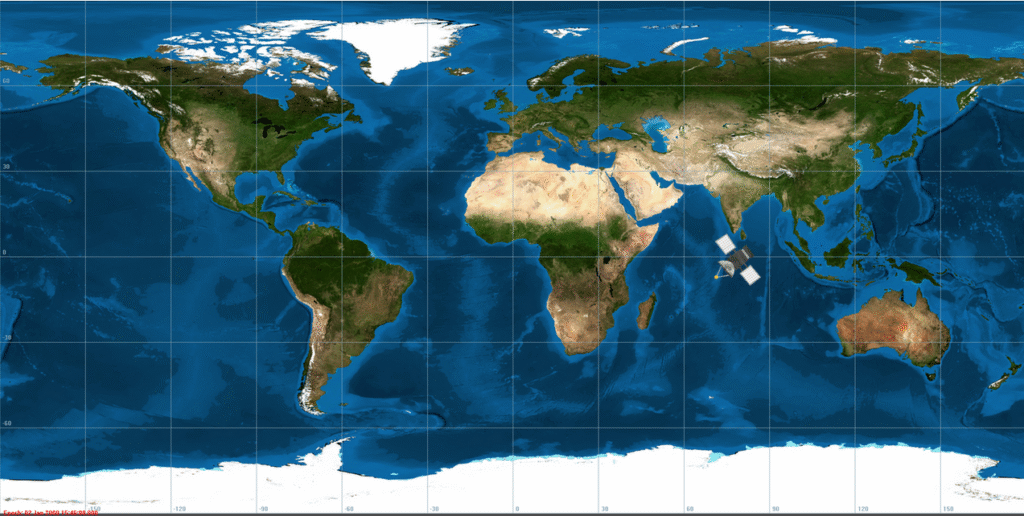
In the picture it is possible to see a ground track image of a satellite in geostationary orbit. It is important to note that the satellite ground track is fixed. This is the result of having the same speed as the Earth! It means that during time, the satellite will be always placed in that position.

Comparison between Low Earth and Geostationary Orbits

Let’s now compare the ground track of a geostationary and LEO orbits. The following picture shows the GEO orbit fixed in a single point and the LEO orbits, in green, that rotates around the Earth. The LEO orbit has been generate considering zero inclination, zero eccentricity and 8000 km radius.

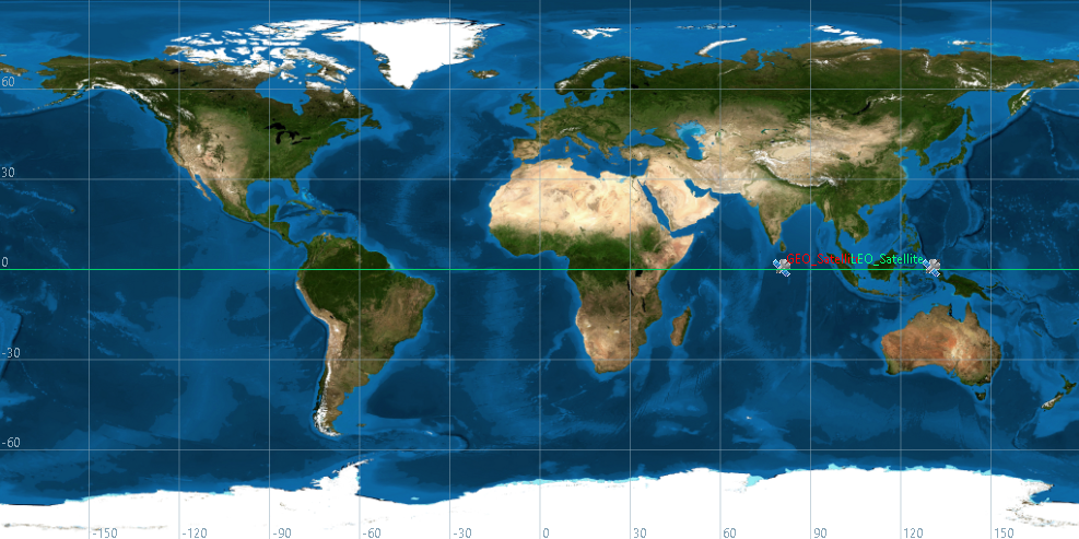
*Ground Track of low Earth orbit (LEO) and geostationary orbit (GEO).*

An interesting comparison is also the orbital period of the two satellites. In fact, we know that the Geostationary Orbit has a period $T = 86,164 \ \text{s}$ . But what a about the LEO period? We can compute that:

$\begin{equation*} T = \frac{2 \pi}{\sqrt{\mu}} r^{\frac{3}{2}} = 7121 \ \text{s} \end{equation*}$

This means that the LEO satellite can complete approximately 12 orbits while the GEO satellite completes just one orbit in the same time. Below a brief video that shows the comparison:

The video shows a simulation that compares between a GEO satellite, whose orbit is represented in red, and a LEO satellite, whose orbit is highlighted in green.

Applications of Geostationary Orbit Equation

Geostationary satellites are fundamental for global communications infrastructure. Because they remain fixed over one spot on Earth, they can provide continuous coverage to a specific region — ideal for real-time communication.

Telecommunications 📡

Satellite Television: GEO satellites broadcast television signals to millions of households. Since their position doesn’t change, ground-based satellite dishes can be permanently pointed at them without tracking.
Internet Access: In remote or not well served areas, without terrestrial broadband infrastructure, GEO satellites offer broadband internet services — though latency is higher than LEO-based systems.
Satellite Phones: Long-distance and emergency communication systems often use GEO satellites to route calls and data in places where cellular coverage is absent.

Weather Monitoring 🌤️

GEO satellites play a critical role also in meteorology due to their ability to observe the same region continuously, capturing consistent, high-frequency images and sensor data. Typical uses are:

Storm Tracking: Meteorological satellites like NOAA’s GOES series monitor hurricanes, typhoons, and tropical storms in real time. Their continuous presence allows for hour-by-hour observation of cloud systems and wind flows.
Climate Observation: Long-term data from GEO satellites contributes to global climate models. They measure variables like sea surface temperature, atmospheric moisture, and solar radiation.
Environmental Monitoring: GEO sensors detect wildfires, volcanic ash, and even aerosol plumes, giving timely warnings to emergency services.

Navigation, Surveillance & Defense 🛰️

Although LEO satellites are more commonly used for high-precision GPS, geostationary satellites complement navigation and are crucial for wide-area surveillance, defense communications, and border security. Typical use cases are:

Military Communication: Secure, high-bandwidth military satellites in GEO provide encrypted communications for ships, aircraft, and ground forces globally.
Disaster Monitoring and Relief Coordination: GEO satellites facilitate coordination between agencies during earthquakes, floods, and large-scale evacuations, thanks to their persistent coverage and communication reliability.
Surveillance and Intelligence: While not as detailed as LEO imagery, GEO platforms can support signal intelligence and persistent wide-area monitoring.

Challenges and Limitations

Despite their advantages, geostationary satellites have several limitations:

Latency – Signals must travel over 70,000 km round trip, introducing a delay of ~240 milliseconds.
Polar Coverage – They can’t see polar regions well due to the equatorial position.
Orbital Congestion – Only a limited number of satellites can operate in the same orbital belt without interference.

In the next sub-chapters we are going to explore the latency and the coverage topics.

Geostationary satellite Latency Estimation

Considering the high altitude of 35 786 km. Signals shall travel for approx 71 572 km.

In the vacuum of space (or nearly so) electromagnetic signals — including radio waves and microwaves — travel at the speed of light: $c = 299,792,458 \ \text{m/s} \ (\approx 3 \times 10^8 \ \text{m/s})$ . Therefore:

$\begin{equation*} \text{Latency}_{\text{one-way}} = \frac{35.8 \times 10^6}{3 \times 10^8} \approx 0.119 \ \text{seconds} \ (119 \ \text{ms}) \end{equation*}$

This is a standard latency if we are sending data that shall cover the Geostationary Orbit Radius distance. An example could be an image captured by the GEO satellite and sent to Ground Station.

Other cases can be the 2-way signals. In this case the geostationary orbit radius shall be covered twice:

$\begin{equation*} \text{Latency}_{\text{round-trip}} \approx 2 \times 119 \ \text{ms} = 238 \ \text{ms}$ \end{equation*}

This is the case of a satellite phone. The scenario could be a phone call, during which we can speak. There will be an uplink to the GEO sat and the voice is download to the receiver in another point of the same are. Obviously, there could be additional steps between.

In this calculation it is computed just the physical signal delay — not including:

Processing delays
Network routing
Atmospheric effects (minimal in GEO cases)

Geostationary Orbit Visibility

At the very beginning of the article we stated that 3 GEO satellites are able to cover a large portion of Earth. Is this really possible? In principle, yes. Due to high altitude the satellites are able to cover a large area. In reality there are some limits due to visibility.

In particular, the transmission from a geostationary orbit becomes less efficient starting from a latitude of 70°. Therefore, for this high latitudes it is necessary to use different orbits.

Let’s analyze more in details the coverage topic.

It is possible to find the geometric limit considering the picture on the right.

$\begin{equation*} R_{\text{GEO}} \cdot \cos(\phi) = R_{\text{Earth}} \end{equation*}$

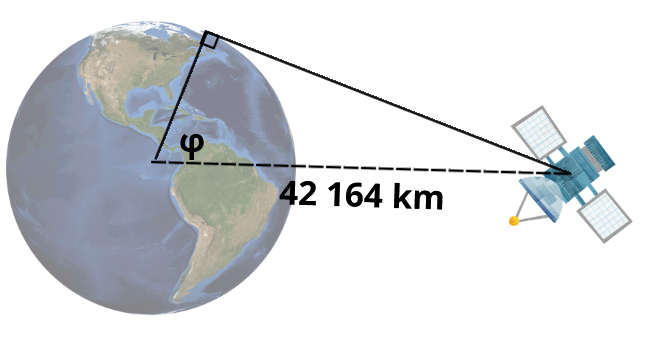
Where:

$R_{\text{Earth}} = 6 378 \ \text{km}$
$R_{\text{GEO}} = 42 163 \ \text{km}$

Therefore, it is possible to compute $\phi$ :

$\begin{equation*} \phi = \arccos \Big( \frac{R_{\text{Earth}}}{R_{\text{GEO}}} \Big)= 81,3° \end{equation*}$

It is possible to state that the geometrical limit is due to the geostationary orbit radius and the geostationary orbit equation, and it is approximately 81,3°. Anyway, as stated before it is possible to find significant loss in terms of coverage since 70°.

Summary

The geostationary orbit equation is a fundamental part of orbital mechanics, allowing engineers to design satellites that hover above one spot on Earth. Solving this equation gives us the radius of geostationary orbit, which is about 42,164 km from Earth’s center or 35,786 km above the surface.

This specific geostationary orbit radius ensures that the satellite remains synchronized with Earth’s rotation, enabling continuous communication and monitoring for regions below.

FAQs

1. What is the radius of geostationary orbit from Earth’s surface?
About 42,164 kilometers.

2. What makes geostationary orbit unique?
It matches Earth’s rotation, keeping the satellite fixed over one point.

3. How is the geostationary orbit equation derived?
From Newton’s law of gravity and the equation for centripetal acceleration.

4. Can geostationary satellites cover the polar regions?
No. Their position above the equator makes them ineffective near the poles.

5. What is the altitude of geostationary orbit from Earth’s surface?
About 35,786 kilometers.

A Comprehensive Guide on Geostationary Orbit Equation, Radius, and Applications

Table of Contents

Introduction to Geostationary orbit equation

What Is a Geostationary Orbit?

The Geostationary Orbit Equation

Calculating the Radius of Geostationary Orbit